

|
Sites > Firebrand
Site: Surveying the fireship Firebrand (1707)
Techniques: 3D Trilateration, Offsets and Ties, Planning frames, Searches, Sketching

The aim of the Firebrand Shipwreck Recording Project was to record the shipwreck of Her Majesty's fire-ship Firebrand which lies under the cold, clear waters off the Isles of Scilly on the south-west tip of England. The archaeological project was a joint venture between CISMAS and Bristol University Department of Archaeology and Anthropology.
The primary aim of the survey work on the fireship Firebrand was to accurately record the positions of the guns, anchors, ship’s structure and artefacts in relation to one another in three dimensions, producing the results as a two-dimensional plan and vertical sections.
Secondary aims were to obtain a position and orientation for the site in the real world, to record the topography and sediment depths on the site and to identify and position any finds around the outside of the main site. An additional aspect of the work was to determine the precision that could be achieved using the methods selected under the given conditions.
All drawings are taken from the Site Recorder file for the Firebrand, courtesy of CISMAS.
Click on any image below to show a larger version.
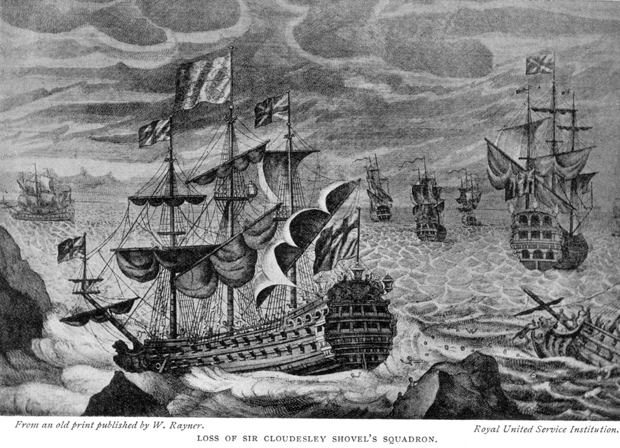
Fig 1: The 1707 Fleet wrecked on the Isles of Scilly
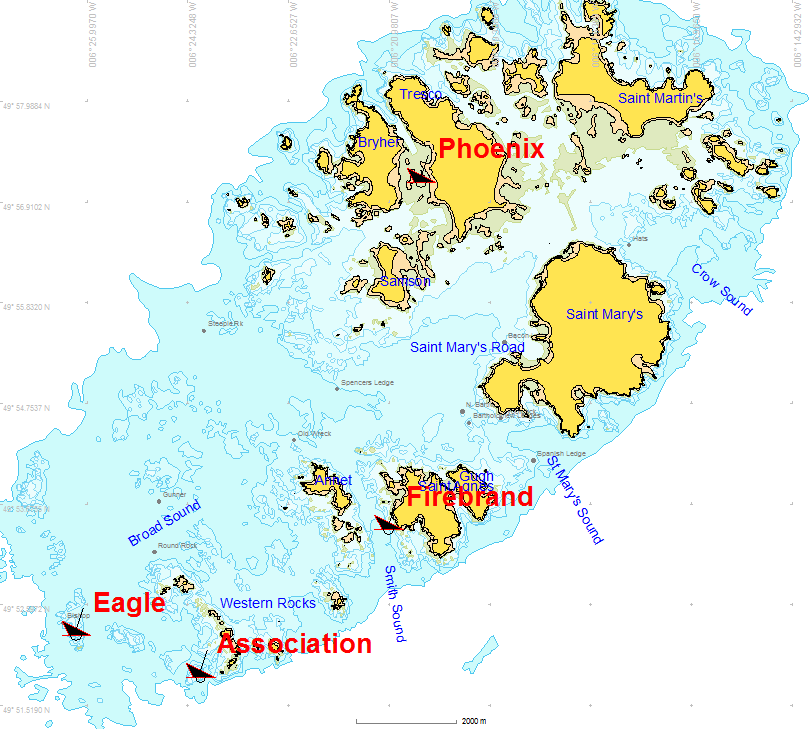
Fig 2: The location of Firebrand and other 1707 Fleet ships as shown in Site Recorder
_1000.jpg)
Fig 3: Dive boat stationed over the Firebrand wreck site
The Site
The wreck of the Firebrand is lies to the west of the island of St Agnes in the Isles of Scilly of the south-west corner of the UK. The shipwreck site is in Smith Sound, approximately 130m west of the shore and 130m south of Menglow Rock in 25 to 27m water depth. The known extents of the site are approximately 45m in length and 10m width aligned 150° / 330°. The remains of the ship are found in a shallow depression formed between a 20m long rock outcrop to the west that runs approximately north-south and the rising slope of the seabed to the east. The seabed in the depression includes sand pockets in amongst large granite boulders and rocks with silty sand at the northern end. Away from the site to the north, east and south the seabed includes large boulders with occasional small sand pockets. The seabed to the north gets shallower as it runs up to Menglow Rock and to the east it shallows towards St Agnes. To the west lies the rock outcrop and beyond this the seabed drops away to 40m at the bottom of Smith Sound. The conditions are typical for a mid-energy site in this area; typical flora and fauna includes wrasse, a sparse covering of seaweed, occasional sea urchins, encrusting sponges and dead men’s fingers.
Requirements
The primary requirement was to accurately record the positions of objects on the seabed by undertaking a pre-disturbance survey of the site. A number of factors would make this task more complicated:
- The main site is large in size but it was still important to maintain sufficient and reliable precision when positioning objects anywhere on the site
- There is a significant difference in depth from one end of the site to the other so any techniques used must be able to compensate for this difference by computing positions in three dimensions
- The depth on site limited dive times to only 30 to 40 minutes so the methods used had to be efficient
- The effect of nitrogen narcosis at depth would also affect the diver’s ability to work underwater so the methods used must be simple and have the potential to detect mistakes in the measurements
- The underwater visibility was approximately 5m which would be considered good for many Northern European sites, but ambient light levels were low at that depth which limited the usefulness of photography or recording
- The budget for the project was small which meant that any newly developed sonar and laser mapping systems could not be used as they were too expensive.
A combination of methods were chosen to record the site based on the limitations given above. Firstly, 3D trilateration was used to set up a network of fixed survey control points around the site then this control point network was then used to position survey detail points on guns, anchors and structure. The site was then drawn in detail using planning or drawing frames positioned using tape measure baselines laid between survey control points.
Although it would have been possible to set up a grid frame over the whole site this would have been more expensive than the chosen method and would have taken a considerable time to set up. A smaller, portable grid frame could have been used but this still requires a precisely positioned control network to position each frame location. Creation of a photomosaic was considered due to the clarity of the water but the low light levels did not give enough contrast to show the details we needed to record. The use of a Sonardyne Fusion acoustic positioning system for precise positioning of artefacts and structure was considered but was beyond the budget of the project.
The Assessment Survey
The first step was to undertake an assessment survey of the site so the information gathered could be used to assist planning the subsequent phases of work. The assessment survey determined the approximate extents of the site, the site’s position and orientation, basic topography, the main visible features and the main seabed types. Assessment surveys should be quick, simple and efficient so this task was completed in a single dive which included a combination of sketching and photography along with a few basic distance and depth measurements. Information from previous site plans was also incorporated and together they formed the basis of a new and very basic site plan that could be used for planning further work.
The assessment survey showed that the site lay in a shallow gully between boulder field to the east and a 20m long rock ridge to the west. The site was approximately 40m long and 10m wide with 25m depth at southern end dropping to 30m at northern end. The seabed was made up of sand and boulders with a scatter of anchors, guns, concretions, a few visible timbers and a few small artefacts.
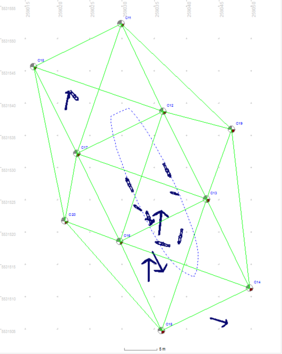
Fig 4: The planned CP network design
The Recording Survey
With the assessment survey completed the recording survey tasks could be started. The methods used for this phase still needed to be efficient but also needed to be detailed and precise so a combination of 3D trilateration and planning frames were used. A set of fixed survey control points (CPs) were set up around the site that were then used to position survey detail points on artefacts and structure and to position planning frames used for detailed recording. The series of tasks undertaken to set up the CP network include:
- Plan the position of the Control Points (CPs)
- Install the CPs
- Make distance measurements between the CPs to be able to position them
- Make a depth measurement at each survey point
- Process the measurements and compute the positions of the CPs using Site Recorder
- Fix the positions of the CPs in the processing software
Planning the Control Point Locations
The next task was to plan the positions for the local survey control point network. The network that was used for this project was designed using basic rules but was adapted to fit with the limitations of the site. The rules for network design are:
- The primary CPs should surround the outside of the site
- Network should be circular or elliptical (with length less than twice the width)
- Made up of sets of four points in a square pattern (‘braced quads’)
- Using distance measurements less than 20m
- Primary CPs should not be installed on artefacts or structure
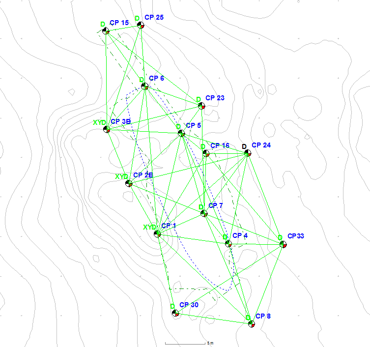
Fig 5: The actual primary control point network design
It is important that the primary control points surround the outside of the site as this ensures that all detail points to be positioned are inside the CP network which gives better results. This also ensures that the primary control points remain undisturbed if the site is excavated or if objects on the site are moved. Where further CPs are needed within the site they are added as extra secondary control points which are not crucial to the main survey network.
The control points should be set out in groups of four in a square or rectangular pattern. This is because the mathematics used to compute positions from distance measurements (trilateration) uses the six distance measurements made between the four points to determine their relative positions and how well they fit together. Networks made up solely of triangles of measurements should be avoided as they do not provide enough information to be able to detect any mistakes in the measurements and so give a poor result.
The network design is based on four interlinked braced quads but because the network is long and thin a pair of ‘outrigger’ points has been added at the sides to provide additional measurements. Each of the braced quads is 15m along each side with diagonal measurements of 21m. The anchor to the south of the site appears to be on its own so was not included in the main CP network as this kept the main network as small as possible which would make it quicker to install (Fig. 4).
Note that only the minimum number of measurements was required as the network shape should be defined by a small number of high quality measurements with enough extra measurements to be able to identify any mistakes. Measuring the distance from every control point to every other point on the site should be avoided as this adds little extra useful information but greatly increases the work to be done and also complicates processing.
On this site the reef to the west of the site severely limited how wide the CP network could be and it also put limits on where the west side CPs could be located. The rounded granite boulders to the east of the site provided few suitable locations for control points so initially the network was set out very close to the guns and anchors on the seabed. The installed CP network was as close tom the planned design as the seabed shape would allow (Fig. 5).
_900.jpg)
Fig 6: Kevin Camidge setting up one of the stainless steel control point pins before installation on the site
Secondary control points were added inside the site. The secondary points were used to provide additional control points for distance measurements to position detail points and they were also used to set up tape baselines through the site used to position planning frames. Each secondary point was positioned relative to the primary network using four or more distance measurements to primary CPs plus a depth measurement.
More about survey control point network design...
Installing the Control Points
The rock ridge that runs the length of the site on the west side was used as the starting point for the primary control point network. Three primary control points (CP1–3) were placed on the tops of rock pinnacles where each would have a good line of sight to the others and to other CPs on the site. Each primary control point was made from a 10mm diameter stainless steel rod 500mm long, stainless steel rod was used so that the points would survive for a considerable time underwater (Fig. 6). Mild steel was only used for temporary secondary points as mild steel rods of similar dimensions were found to corrode within 18 months if placed near iron objects like guns or anchors. Tape measures can easily be attached to these rods using releasable cable ties/tie wraps.
Each rod installed on rock was hammered and cemented into a fissure in the top of the rock. The cement used for this was a mixture of 3 parts sand to one part Portland cement, with a small amount of PVA glue added to bind the mixture together and enough fresh water to give the mixture the consistency of toothpaste. The mixture was made up on the boat just before the dive and put in small polythene bags in handful amounts. Underwater, the cement bags go stiff under the water pressure so have to be pushed and hammered into the crack which will take the control point pin. The pin itself can then be hammered into the crack through the plastic bags full of cement. Any cement or bag visible should be covered in small stones or gravel to stop it washing away, and once the cement has set any plastic bag still visible can be removed.
Installing CP30 was unusual as a chisel mark on the top of a very large granite boulder was used to mark the survey point as no other location was suitable and it was not possible to attach anything directly to the boulder.
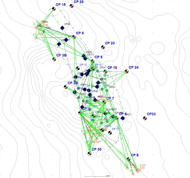
Fig 7: Detail survey points positioned from the control points
Each point was labelled with a yellow Disk-mark tag and a length of yellow flagging tape was tied around the top of the rod to make the points more visible. Survey points were named in sequence starting with CP1 (Control Point). Primary and secondary points use the same naming format for convenience and as the role of any point could change as the survey work progressed.
More about installing survey points...
The Installed Network
In the 2006 season the primary control points CP1 to CP8 were added to the site. In 2007 we found that the pins marking CP2 and CP3 had been removed since the last visit to the site so they were replaced with points CP2B and CP3B in new positions close to the original locations. The new points were given names similar to those they replaced but different names were used as the replacements were not in exactly the same place as the ones that had been removed.
The primary point CP12 was added in the middle of the site along with secondary points CP9 to CP11. In 2008 the primary point CP15 was added to extend the site to the North and CP30 to extend it to the South. Points CP16, 23-25 were added to the East of the site to improve the network shape by making it wider. In 2009 point CP33 was added to strengthen the network at the south end of the site.
Secondary points CP17, 20 and 31 were added to support the planning frame survey and were left in place. Secondary points CP18, 19, 22, 26, 27, 28, 29, 32 were added for the same reason but were subsequently removed.
The positions on the site are recorded with Z positive downwards so Z measurements are given as depths. All depths are reported relative to a temporary benchmark (TBM) defined as the top of the cascabel of Gun 1, at survey detail point G1c. This point was given a fixed value of 25m and all depth measurements have been corrected for the effects of tide height using this point.
Making Measurements
With the control points in place the next step was to measure the distances between the points based on the network design shown above. Distance measurements were made using conventional builder’s fibreglass tape measures, less than 30m long with open frames so they could be washed after use. As tape measures can stretch with use, each tape was checked for accuracy against a steel-cored tape measure kept solely for this purpose. Measurements were recorded in millimetres standard recording forms.
_800.jpg)
Fig 8: The Firebrand team processing the day's drawings using Site Recorder
Depth measurements were made using a Suunto Vyper digital dive computer and a single computer was used for all depth measurements to minimise offset errors. The range of tide on site is up to 5m so all depth measurements had to be corrected by having the tide height removed. To do this, one point was nominated to be the depth reference point and was given a nominal depth. Before any depth measurements were made at other points the depth and time were first recorded at the depth reference so the height of tide at that time could be calculated. Depth and time measurements were then made at other points, finishing off with another measurement at the reference point so we could calculate the change in depth during the dive. The tide height at the time each other depth measurement could then be calculated from the two depth measurements and times recorded at the reference point, and the calculated tide height could then be removed from each raw depth.
Position measurements were used to locate the site in real-world co-ordinates and to calculate the alignment of the site. Surface buoys on ropes were attached to two known points at the extreme ends of the site, using points far apart would provide a long baseline between the points and this would increase the precision of the alignment. Surface positions were taken using a WAAS enabled Garmin 76C GPS receiver. The estimated position error for a static fix at the surface using this receiver is 4m however additional offset error will occur because of the rope attaching the buoy to the seabed.
The site was moved and aligned to these positions so that the crown of Anchor 5 was at the position GPS001 and the cascabel of Gun 1 was placed as close as possible to GPS002. The position of the cascabel computed from the trilateration survey differs from the GPS fix by only 3.6m, a small difference given the errors associated with this method.
More about positioning using GPS...
Processing
The positions of the primary survey control points were calculated by combining the distance, depth and surface position measurements using Site Recorder 4 (Fig. 8). The program calculates the best estimate of the position of the points, an estimate of the position error for each point and calculates quality metrics for each of the measurements using a survey quality least-squares adjustment. Any measurements that were found to be in error were re-measured and the point positions recalculated. As the surface position measurements were included in the position calculation the computed positions for the points were automatically given in real-world co-ordinates.
_800.jpg)
Fig 9: Using a drawing frame on site
The estimate of error used in the adjustment for distance measurements was 30mm and for depth measurements it was 100mm. After adjustment, the 71 measurements made between the 16 primary control point fit together to within 21mm (RMS of residuals) horizontally and 30mm in the vertical. A total of 119 measurements were processed together to position the 41 primary and secondary points giving an overall RMS of 16mm. These results are as expected for a survey of this type under the conditions found on site.
All positions are given using the WGS84 datum and grid positions use the Universal Transverse Mercator (UTM) projection Zone 30N.
Positioning Detail Points
Once the positions for the primary control point network had been calculated, these CPs were used to position detail survey points on guns, anchors and artefacts (Fig. 7). To position each detail point, measurements were made from each detail point to the four primary control points nearest to it. Where not enough primary points were within a close enough distance a measurement was made to a suitable secondary control point instead. A depth measurement was also made at each detail point.
Guns were positioned using two detail points, one on the top of the cascabel and the other the top of the front face of the muzzle. The name of each detail point included a ‘G’ prefix, the gun number and either ‘c’ for cascabel or ‘m’ for muzzle (for example, the two points on Gun 6 were G6c and G6m). Anchors that were intact were positioned using four detail points, one on the shank, one on the crown and one on each of the two flukes. The name for each detail point included an ‘A’ prefix, the anchor number and one of four identifiers for each location ‘S’, ‘C’ ‘fW’ and ‘fE’ (for example, Anchor 4 used the four points A4S, A4C , A4fW, A4fE). Small artefacts were positioned using a single detail point.
The adjustment of the positions of the detail points positioned from the fixed control network gave an RMS of residuals of 24mm.
Recording using Drawing Frames
Drawing or planning frames were used to record a plan view of the site in two dimensions. If a drawing frame grid is laid on the site in a known location the seabed under it can be drawn to scale by a diver and that drawing can then be replicated to scale on the site plan (Fig. 9), if this is done across the whole site the separate drawings can be stitched together to form a complete site plan (Fig. 10 &11).
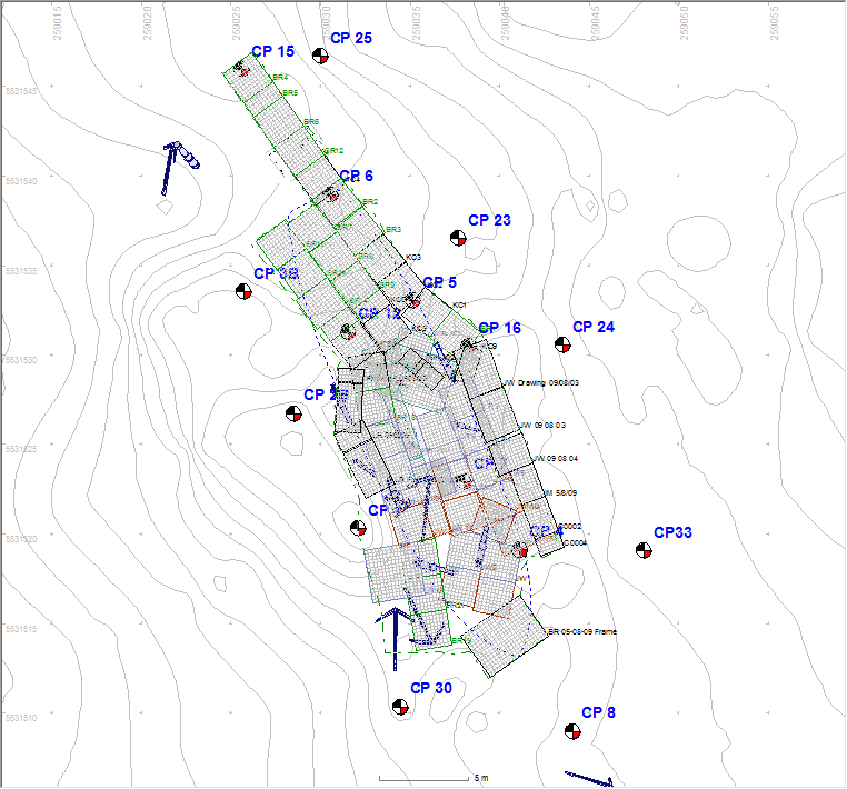
Fig 10: The planning frames used to record the site
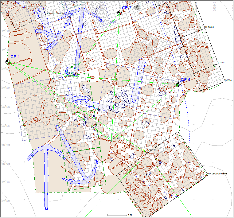
Fig 11: Detail of the planning frames at the south end
To maintain precision in the site plan the drawing frames need to be accurately positioned. Drawing frames were positioned relative to a tape measure baseline set up between two CPs or occasionally they were positioned relative to two or more survey points. Where a baseline was used to position the frame the two points where the tape crossed the edge of the frame were recorded on the drawing along with the distance along the tape baseline of one of those crossing points. The positions of any survey points were also recorded on the diver’s drawing so these could be used to position the frame or as an additional cross-check on position accuracy.
Processing the drawing frames was also done using Site Recorder directly onto the digital site plan. For each drawing frame drawn underwater a Drawing Frame object was added to the Site Recorder file and positioned on the chart using a baseline (Distance Measurement) or two survey points. For each frame the points where the baseline crosses the edge of the frame was defined so it would automatically position itself on the site plan in the correct location. The drawing made underwater was then scanned and added to the appropriate Drawing Frame in Site Recorder where its image was then shown on the chart at the correct scale and in the right location and orientation. The scanned drawing was then traced (digitised) separating rock, concretion and timber onto different drawing Layers. As a final step, the traced lines between adjoining frames were joined together by hand to make a seamless site plan (Fig 12 &13).
Click here for a high-resolution interactive site plan of the Firebrand fireship...
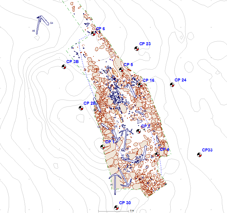
Fig 12: The resulting plan of the Firebrand site
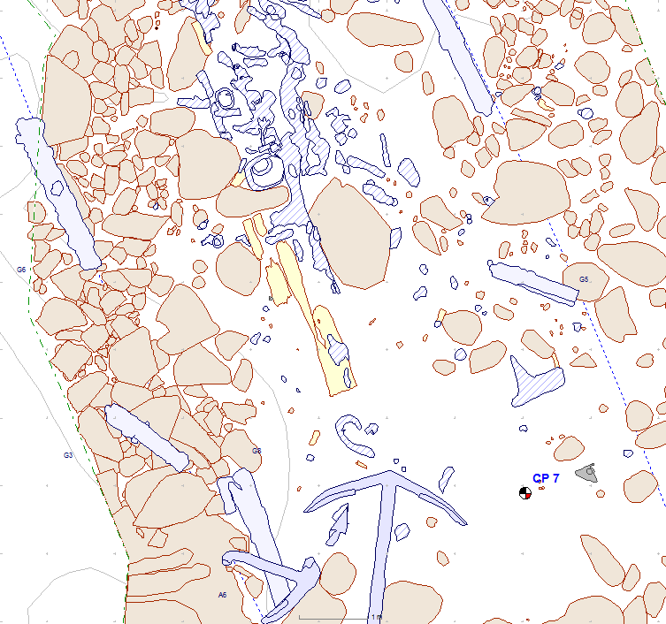
Fig 13: Detail view of the site plan
Area search, Probing and Topography
The shape of the seabed on the site is likely to have played a part in how the site was formed as the wreck appears to have settled between two rock reefs so the shape needed to be recorded. The shape of the seabed was estimated using depth profiles measured across the site, these are lines of depth measurements made between two known points (Fig. 14). Each depth measurement could then be plotted on the site plan and together they were turned into a contour plot. Depth measurements were made using a dive computer and were corrected for the effects of tide. Distance measurements were made using a tape measure attached to a control point and run out at a known bearing, or using a Sonardyne Homer Pro beacon locator in place of the tape measure. The depth points were exported from Site Recorder to a file in XYZ format then were used to create a contour plot of the site bathymetry using Surfer (Fig. 15).
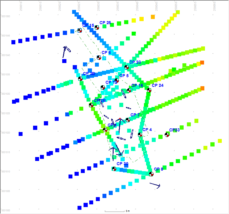
Fig 14: Depth transects measured across the site
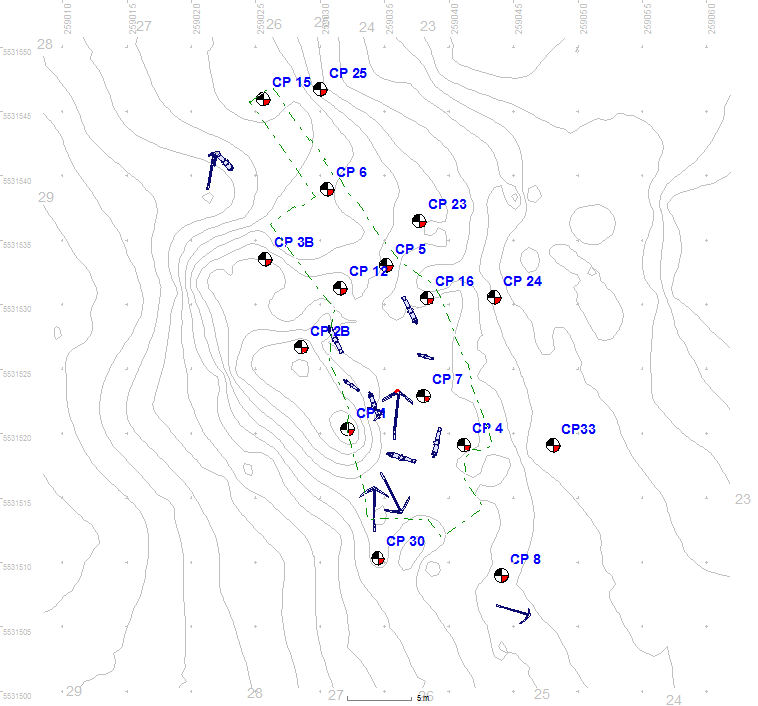
Fig 15: Seabed depth contours
The sandy areas of the site were searched for the presence of any metal objects buried beneath the surface using a pulse induction metal detector. The targets located during the search were positioned using offset measurements from baselines laid between survey points then plotted on the plan in Site Recorder (Fig. 16)
Another task was to search the immediate area around the main site and to position any artefacts that were found. The aim was to asses the quantity of finds and to see if there were any groups of objects that needed further investigation so precise positioning was not requried. Radial measurements were used to position the artefacts found during the area search; a tape measure was laid from a nearby control point to each artefact and the distance measured along with the back bearing along the tape to the CP. The distances and bearings were processed in Site Recorder as Radial measurements so could be directly plotted on the site plan (Fig. 17).
More about radial measurements...
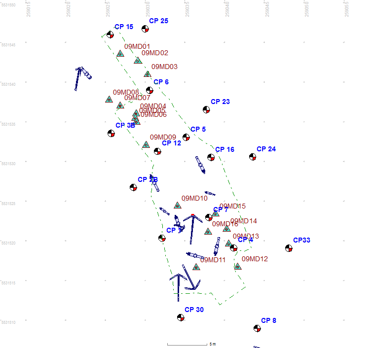
Fig 16: Metal detector targets
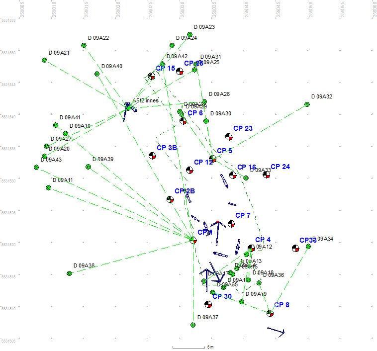
Fig 17: Finds around the main site positioned using radial measurements
Site Data Management
The project was managed during the planning, data collection and post-processing phases using Site Recorder 4 (SR4). The program was used to increase working efficiency, minimise paperwork and to allow data sharing and publication.
Site Recorder was used during the planning phase undertaken before fieldwork started to collect together all of the information we had about the site and its surroundings. This included digital charts of the area and previous site plans on paper scanned and included as georeferenced basemap images.
During each season’s fieldwork the program was used to record and process distance, depth, position and radial measurements used to position control and detail survey points on the site. The planning frame drawings made each day were scanned, added to Site Recorder and digitised each evening so each morning we knew if any work needed to be added to or repeated. Finds were added to the archive as Artefact objects along with Sectors to represent trenches and a Sample added for each sample taken. The archive also included linked documents, dive logs, information about divers and 16 metal detector targets.
During the post-processing the raw data collected during the fieldwork was cleaned, processed and rendered on the plan. The data in Site Recorder was then used as primary information source during the creation of the site plan, AutoCAD was used to create the fair sheet site plans using data exported from SR4 as a DXF file.
The entire digital archive of information about the site is available as a Site Recorder file that can be viewed using the free Site Reader program. Later work on the site can reuse this digital archive using a copy of Site Recorder or by incorporating data exported from the archive into another data management program.
Survey Precision Analysis
More about the analysis of the survey accuracy...
Conclusion
In summary, the methods used for this project were a good compromise between precision and cost.
The achieved precision was similar to the computed precision so the results were as expected for this type of survey. A more precise result could have been achieved by taking additional distance measurements to those points with only three measurements, using a more precise method for measuring depth, more care in positioning planning frames or by using a different method to position them.
However, the site is 46m long by 15m wide and it has been disturbed by salvors so an estimated achieved precision in the order of 100mm is acceptable. There may be little more useful information to be gained by doing a more precise survey on this site, but the cost of the project would have increased significantly.
Related Pages
- Firebrand survey accuracy analysis
- 3D Trilateration
- Planning frames
- Radial measurements
- Metal detectors