
Research Techniques > Research > Tape Measure Accuracy
- How Accurate are Tape Measure Surveys?
Version date: 23 October 2016
Introduction
The results of this experiment were originally published in the International Journal of Nautical Archaeology as An Assessment of Quality in Underwater Archaeological Surveys Using Tape Measurements, IJNA (2003) 32.2: 246-25 1. The version here has been updated and expanded slightly.
The Problem
One of the first experiments we did into the science of underwater surveying was to find out how accurate tape measure surveys were when done underwater. At the time it was thought that because tape measurements were made to the nearest millimetre the accuracy of the survey was to the nearest millimetre as well. Unfortunately this ignored the problem of measurement error so a test was devised to work out what the accuracy of tape measure surveys really was.
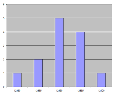
Fig 1: Histogram of tape measurements made on land
The problem with tape measurements can be seen in Figure 1. A set of 13 tape measurements was made by archaeology trainees over a distance of 12.4 m on land, with the tape unsupported but with no wind to move the tape. Five of the measurements were 12.390m, four were 5mm longer and one was 10mm longer, while two were 5mm shorter and one was 10mm shorter. If only one measurement was made then the value could be between 12.380m and 12.400m, giving a spread of 20mm even though the measurements were recorded to the nearest millimetre!
We can calculate the most likely value for the measurement using statistics. The average value is also the most frequent at 12.390m and the spread we can define using a value called standard deviation which works out at 6 mm. None of the values was wrong as you would expect from tape measurements made over a short distance on land in ideal conditions.
The Experiment
What we needed to do was to find a way to work out how good tape measurements were when made underwater in not idea conditions. We could simply repeat this test and get lots of divers to make the same measurement, but this would hide other factors that may affect the result. What we needed was a way of calculating the quality of a set of tape measurements made on an entire site.
The test had to produce a single average accuracy value for an entire survey so measurements needed to be made over a varying range of distances. The measurements would also contain errors as divers make mistakes when recording so the experiment needed a way of sorting the real measurements from the mistakes. 3D trilateration was chosen for this test as the required quality information is produced as a by-product of processing the measurements. The measurements are processed together to compute a best estimate of the points the measurements are made between, then the measurements can be compared to see how well they fit together. The standard best-fit process is called least squares, this gives the most desirable result (one with the highest precision) and is very simple to calculate (Cross, 1981; Atkinson et al., 1988; Bannister, 1994). 3D trilateration is often called the 'Direct Survey Method' and was popularised in marine archaeology by Nick Rule (Rule 1989). The methods used for processing distance measurements is similar to that used by Global Positioning System receivers (UKOOA 1994) and underwater acoustic positioning systems (Kelland 1994).
Test Site
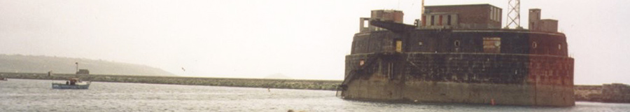
To calculate the quality metrics we needed a sample data set of multiple sets of tape measurements made between a number of fixed and rigid points on a typical site underwater. No corrections were applied to the measurements for temperature, sag or tension so the results would be close to those achieved on a typical underwater site. As a suitable site was not available a test site was set up in 1996 at the base of the Breakwater Fort behind the Breakwater in Plymouth Sound, described in the Case Studies. This site was used by the Fort Bovisand Underwater Centre as a training ground for commercial divers as it was sheltered, only 10 m deep, had minimal current and had underwater visibility between 2 m and 5 m.
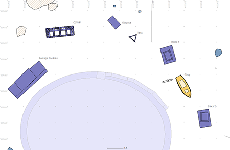
Fig 2: Site plan of the Breakwater Fort, Plymouth

Fig 3: Three-dimensional model of the Breakwater Fort site
The chosen site contained a number of fixed and rigid structures suitable for recording. These included two large concrete blocks, the wall of the Fort itself (Fig. 2, Fig. 3) and a 7 m long ex-Pilot cutter called Tavy which had been sunk deliberately for this experiment. A network of 21 control points was installed on the structures (Fig 4), the shape was designed to give a large amount of redundancy and minimal sensitivity to errors in depth measurements. The control points installed on the structures were 5mm galvanised coach bolts cemented into pre-drilled holes; the diameter of the control point bolts was accounted for within the processing program.
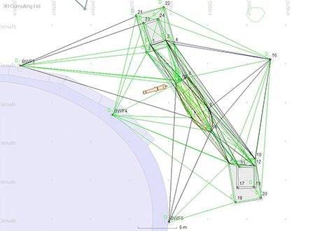
Fig 4: Measurements between the 21 control points
Over a period of a year many teams of divers recorded a pre-defined set of measurements between the control points to 1mm resolution using the same set of tape measures for each exercise. As a check for systematic errors, all tape measures were calibrated against a steel-cored tape measure at 5 m, 10 m and 20 m distances and any tape measures with more than 5 mm in error were not used. To minimise transcription errors, standard recording forms were used and the data was transferred from the form straight into the computer for analysis.
Results
A total of 32 baselines with distances between 2 m and 13 m were measured more than 5 times, comprising a total of 178 measurements. Another 85 baselines which had less than 5 measurements each were included giving 304 measurements in total. The measurements were processed using the least-squares method implemented in Site Recorder which calculated the best estimate of position for each survey point. The program then calculated the best estimate of distance between each point and compared that to the actual measurements. The difference between the calculated distance and each measurement is called a residual, and for the measurements to be good then the residuals will be zero or very small.
The majority of the baselines showed one or more gross errors even though some lengths were less than 3 m. For example, Figure 5 shows the residuals for 12 measurements of a baseline just 1.7 m long (CP5 to CP6) where 11 of the measurements agree with the calculated distance to less than 20 mm but one is in error by nearly 140 mm. Measurements like this that are much too short or much too long are known as outliers, see Measurement Errors.
With the obvious outliers removed the mean and standard deviation of the measurements was calculated for each baseline. Together the baselines gave an average standard deviation of 25 mm where the minimum was 8 mm and the maximum was 60 mm. This value for precision of 25 mm was used as the starting point for subsequent analysis.
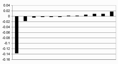
Fig 5: Measurement residuals for baseline 5-6 with one large outlier
Figure 6 shows the residuals plotted in size order with a vertical bar showing the approximate point of separation between valid measurements to the left and outliers to the right. Many large outliers existed in the data set, but as can be seen from Figure 6 there was no clear distinction between the valid measurements and the start of the outliers. Two methods were used to identify outliers, the first was to manually reject any measurements over a given limit, here a rejection limit of 3 standard deviations (99.7%) was used with our previously computed precision of 25 mm, so any outlier larger than 75 mm was rejected. The second method was to use an automatic rejection process based on the Delft method recommended for processing GPS measurements (Table 1). The automatic rejection method is an iterative process that rejects the measurement with the highest w-statistic or normalised residual after adjustment. The process stops when all remaining w-statistic values lie below 2.576 or 99%. The normalised residual is obtained by dividing a residual by its standard deviation so both the manual and automatic methods are driven by our estimate of precision.
Rejection |
None |
3 S.D. |
Delft |
RMS of the residuals |
143 mm |
30 mm |
27 mm |
Measurements |
304 |
304 |
304 |
Measurements used |
304 |
247 |
240 |
Measurements rejected |
0 |
57 |
64 |
Measurements rejected |
0 % |
18.8% |
21.0% |
Table 1: Post adjustment results
Of the 304 observations, 168 (55%) were smaller than the defined measurement standard deviation and 57 were larger than 3 times the standard deviation. The Root-Mean-Square (RMS) of residuals gives an idea of how well all the measurements fit together, in the case where no outliers were rejected the RMS value was 143 mm showing that outliers existed in the data set. In the cases where outliers were rejected the RMS of residuals becomes close to the expected value of 25 mm, our nominated precision for the measurements. It was expected that longer measurements would be more likely to have larger residuals however the data shows that this is not the case.
Curiously, the set of residuals shows no correlation between measurement length and residual (Fig. 6) as it was initially thought that shorter distances would be more likely to be correct. The black line in the figure shows the length of each measurement and there are as many long distance measurements as short ones spread across the graph. So for measurements up to 20m the long measurements were just as likely to be correct as the short ones.
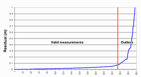
Fig 6: Measurement residuals in residual size order
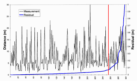
Fig 7: Raw measurements and residuals in residual size order
Knowing the typical precision of a tape measurement we can calculate the accuracy with which we can position any point on the site. The accuracy of the position of a point is expressed as error ellipse based on both the precision of the associated distance measurements and the position of the point within the control network. The ellipse is an approximate graphical representation of the horizontal accuracy in all directions. Error ellipses are commonly shown at 2.447 times their 1 SD values and are then referred to as 95% confidence regions, so there is a 95% confidence that the point lies within that ellipse. The sizes of the error ellipses computed by the adjustment program are directly related to the size of the standard deviation defined for the tape measurements. The standard deviation also sets the maximum acceptable residual so a small standard deviation gives a small size of error ellipse but requires better quality measurements to achieve it. A simulated network of four fixed control points was set up with a test point A in the centre, Test B on a baseline between two control points and Test C outside the control network (Fig. 8). The position error ellipses are shown 20 times full scale. The accuracy of the position of a set of points was then calculated based on the given precision of 25 mm (Table 2).
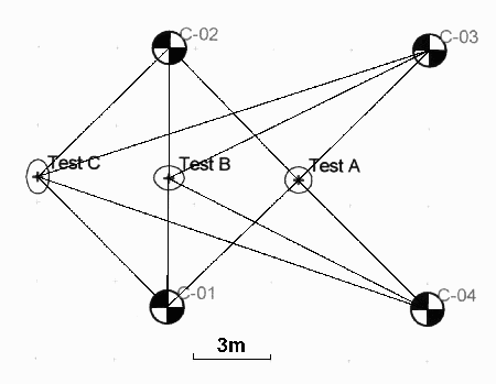
Fig 8: Position precision test
|
Semi-Major (95%) |
Semi-Minor (95%) |
Note |
Test A |
43 mm |
43 mm |
Centre of the network |
Test B |
48 mm |
39 mm |
Between two control points |
Test C |
56 mm |
37 mm |
Outside the control points |
Table 2: Point accuracy results
As a cross check on the 25mm SD value calculatede for this survey, measurements from a number of other similar underwater sites were processed in order to obtain an estimate of the distance measurement precision and the percentage of outliers in the data set (Table 3). In each case the automatic rejection tool in Site Recorder was used. The RMS residual values of between 10 mm to 25 mm are typical for shallow water sites.
|
Control points |
RMS Residuals |
Outliers |
Hazardous |
12 |
8 mm |
8 of 52 15% |
Boyne |
21 |
15 mm |
8 of 101 8% |
Resurgam |
12 |
17 mm |
5 of 45 11 % |
Coronation |
12 |
8 mm |
0 of 39 0% |
Colossus |
18 |
23 mm |
10 of 125 8% |
Alum Bay |
14 |
10 mm |
9 of 77 12% |
Table 3: Residuals and outliers from other sites
Conclusions
Under the test conditions, a standard deviation of 25 mm is valid for measurements made underwater using fibreglass tape measures over distances up to 20 m. This value can be used as a typical figure for tape measurements under similar conditions. The single data set on land showed a standard deviation of 6 mm over a comparable length. The cause of the difference between land and underwater measurements is most likely to be a combination of the effects of any water current on the tape and inability to maintain the correct tension on the tape when underwater.
The number of outliers in the test data set was approximately 20%, considerably larger than is usually assumed for survey work underwater. This high percentage of outliers emphasises the need for making extra redundant measurements and highlights the need for appropriate survey data processing techniques to identify and eliminate the outliers. The tests were done using 3D trilateration measurements however it is likely that the same number of outliers will occur when positioning using offsets and ties as the same measurement procedures are used. There were outliers even in short baselines where the tape was supported along its whole length. It is unlikely that stretching in the tape caused these outliers, the more likely cause was mis-reading of the tape measure or transcription errors when transferring measurements to the recording forms or from the forms to the computer.
There was no obvious correlation between size of outlier and measurement length so large outliers are as likely to appear in short measurements as long ones. This result was unexpected and hints that a significant proportion of the outliers came from mis-reading or transcription errors. This is important, as it means that such problems can be minimised with diver training and reducing the number of transcriptions. Where a diver is in voice communication to the surface, fewer mistakes will probably be made if the surface team rather than the diver record the measurements. The best method appears to be to process measurements on the computer as they are made allowing the immediate identification of outliers as this minimises the amount of re-work to be done.
The post-computed position confidence regions for points inside the control network can be approximated to circles 40 mm in radius. This means a typical point positioned using 3D trilateration with tape measures will be accurate to ±40 mm at 95% confidence. This figure can be used as a baseline standard for comparison with other methods of positioning underwater such as acoustic or optical systems under similar conditions. These tests were done under almost ideal conditions for UK waters and the precision achieved is likely to be the highest achievable, so the next step would be to repeat the tests under more taxing conditions.
References
- Atkinson, K., Duncan, A., and Green, J., 1988, The application of a least squares adjustment program to underwater survey, IJNA 17.2: 119-131
- Bannister, A., Raymond, S. and Baker, R., 1994, Surveying, Prentice Hall, ISBN 978-058 2302 49 5
- Cross, P. A., 1981, The Computation of Position at Sea. Hydrographic Journal 20
- Holt P., 2003, An Assessment of Quality in Underwater Archaeological Surveys Using Tape Measurements, IJNA 32.2: 246-25 1
- Kelland, N., 1973, Assessment Trials of Underwater Acoustic Triangulation Equipment. IJNA 2.1 : 163-176
- Kelland, N., 1994, Developments in Integrated Underwater Acoustic Positioning. Hydrographic Journal 71
- Rule, N., 1989, The Direct Survey Method (DSM) of underwater survey, and its application underwater, IJNA 18.2: 157-162
- UKOOA, 1994, The Use of Differential GPS in Offshore Surveying, UKOOA